Image of spherical black hole with thin accretion disk

April 20, 2025

by Jean-Pierre Luminet 1979

Abstract

Black hole accretion distks are crretnly a topic of widespread interest in astrophysics and are suppose to play and important role in a number of high-energy situations. The present paper contains an investigation of the optical appearance of a spherical black hole sourrounde by a thin accretion disk. Isoradial curves corresponding to photons emitted at constant radius from the hole as seen by a distant observer in arbitrary direction have been plotted, as well as spectral shifts arising from gravitational and doppler shifts. By the results of Page and Thorne (1974) the relative intrisinc intensiy of radiation emitted by the disk at a given radius is a known function of the radius only, so that it is possible to calculate the exact distribution of observerd bolometric flux. Direct and secondary images are plotted and the strong asymmetry in the flux distribution due to the rotation of the disk is exhibited. Finally, a simulated photograph is constructed, valid for black holes of any mass accreting matter at any moferate rate.

Introduction

In order to be visible a black hole has of course to by illuminated, like any ordinary body. One of the simplest possibilities would be for the black hole to be illuminated by a distant localized source which in practice might be a companion star in a loosely bound binary system. A more interesting and observationally important possibility is that in which the light source is provided by an emitting accretion disk around the black hole, such as may occurt in a tight binary system with overflow from the primary, and perhaps also on a much larger scale in a dense galactic nucleus. The general problem of a the oprical appearance of a black hole is relared to the analysis of trajectories in the gravitational field of black holes. For spherical, static, electric-free black holes (whose external space-time geometry is described by Schwarzschild metric) this problem is already well know (Hagihara, 1931; Darwin, 1959; for a summary, see Miner etal. 1973 MTW). In Sec. 2 we give only a brief outline of it with basic equations, trying to point out the major features which appear latter. All our calculations are don in the geometrical optics approximation (for a study of wave-aspects, see Sanchez, 1977). In Sec. 3 we calculate the apparent shape of the circular rings orbiting a non-rotating black hole and the results are depicted in Figs. 5-6. In Sec. 4 we recall the standard analysis by Novikov and Thorne (1973) of the problem of energy release by a thin accretion disk in a general astrophysical context, focusing attention more particularly on the analytic solution for the surface distribution of energy release that was derived by Page and Thorne (1974) in the limiting case of a sufficiently low accretion rate. In terms of this idealized (but appropriate circumstances, realistic) model, we calculate the distribution of bolometric flux as seen by distant observers at various angles above the plane of the disk (Figs. 9-11).

Images of Bare Black holes

Before analyzing the general problems of a spherical black hole surrounded by an emitting accretion disk, it is instructive to investigate a more simple case in which all the dynamics are already contained, namely the problem of the return of ligth from a bare black hole illuminated by a light beam projected by a distant source. It is conceptually interesting to calculate the precise apparent pattern of the reflected light, since some of the main characteristics features of the general geometrical optics problem are illustrated thereby.

The Schawarzschild metric for a static pure vacuum black hole may be written as

\[ds^2 = -\left(1-\frac{2M}{r}\right)dt^2+\left(1-\frac{2M}{r}\right)^{-1}dr^2+r^2\left(d\theta^2+\sin^2\theta d\varphi^2\right)\quad(1)\]

where \(r\), \(\theta\) and \(\varphi\) are spherical coordinates and the unit system is chosen such that \(G=c=1\). \(M\) is the relativistic mass of the black hole (which has dimenssions of lenght). In this standard coordinate system the horizon forming the surface of the hole is located a the Schwarzschild radius \(r_s=2M\), see Eq.(1).

One can take advanange of the spherical symmetry to choose the equatorial plane \(\theta=\pi/2\) so as to contain any particular photon trajectory under consideration. The trajectories will then satisfy the differential equation (See derivation equation 2):

\[\left(\frac{1}{r^2}\left(\frac{dr}{d\varphi}\right)^2\right)^2+\frac{1}{r^2}\left(1-\frac{2M}{r}\right)=\frac{1}{b^2}\quad(2)\]

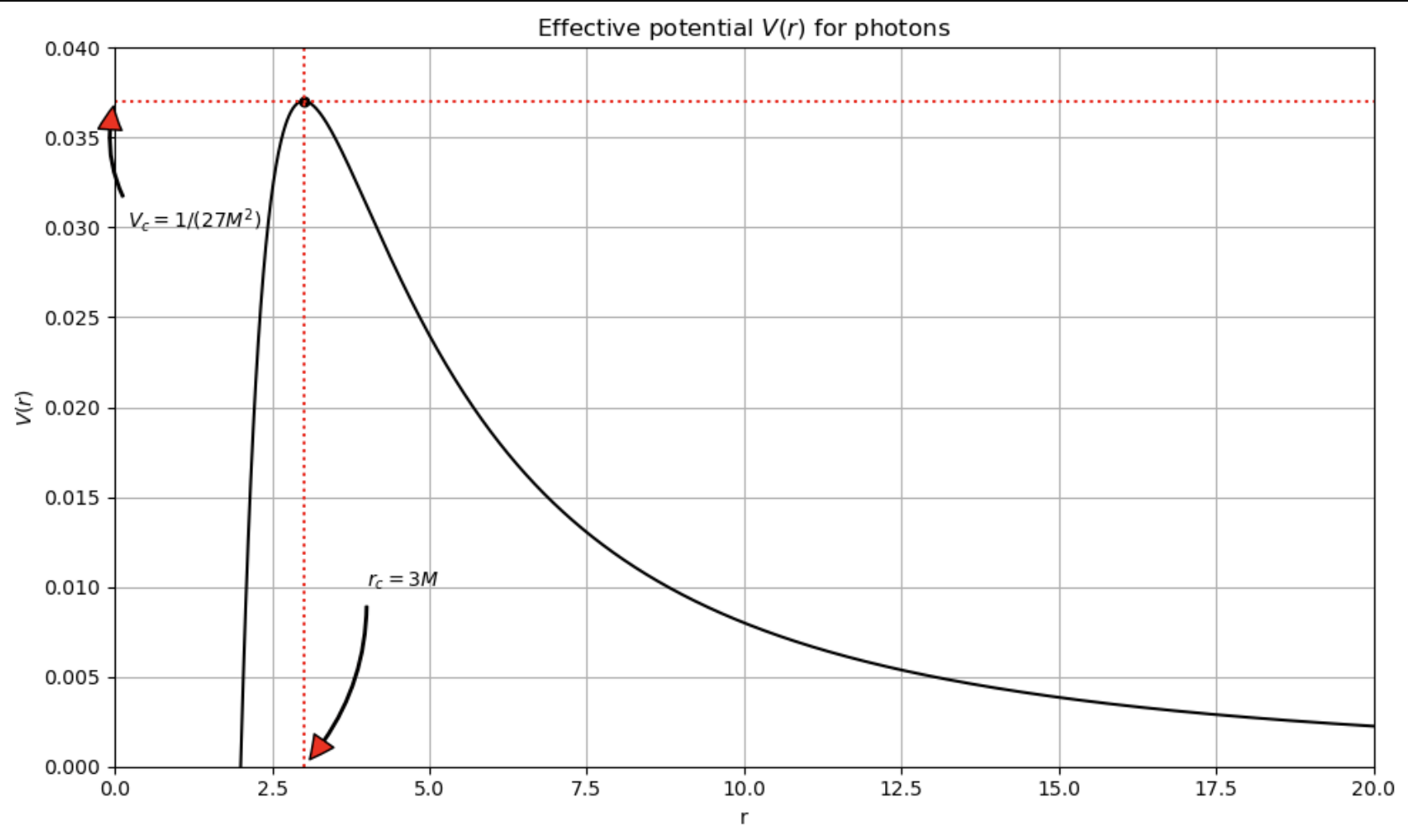
The second term in the left member can be interpreted as the effective potential \(V(r)\), in analogy with the non-relativistic mechanics. The motion does not depend on the photon energy \(E\) and on its angular momentum \(L\), but only on the ration \(L/E=b\), which is the impact parameter at infinty.

Let the observer be in a direction fixed by the polar angle \(\varphi_0\) in the Schwarschild metric, at a radius \(r_0>> M\) (the observer is at infinity). The rays emitted by a distance source of light deflected by the black hole intersect the observert’s detector (for example a photographic plate) at a distance \(b\) from the the central point of the plaque. From (2), one sees that a ray with impac parameter \(b\) can reach a point at a distance \(r\) ony if \(b\leq [V(r)]^{-1/2}\). This can be seen directly from (2), from which

\[\frac{1}{r^2}\left(\frac{dr}{d\varphi}\right)=\sqrt{\frac{1}{b^2}-V(r)}\]

It is clear that the rim of te ‘‘optical’’ black hole corresponds to rays which arre marginally trapped by the balck hole: the spiral around many times before reaching the observer, and in our case the rim (borde) is located at \(b_c= 3\sqrt{3M}\approx 5.19695M\). Thus, the apparent diameter of the hole is about \(10.38\).

'''
We began by defining the black hole mass M, the Schwarzschild radius r_s (horizon), 
the photon radius r_c (critical radius), the critical impact parameter b_c, and the function effective potential. 
We use geometrized units and create an arrange of values for r.
'''
M   = 1
r_s = 2*M
r_c = 3*M
b_c = 3*np.sqrt(3)*M
radial_coordinate = np.arange(r_s,100, 0.01)
"""
Definition of the effective potential
"""
def V(r):
    Veff = (1/r**2)*(1-r_s/r)
    return Veff

Let usreturn to Eq. (2). Letting \(u=1/r\), we get (See derivation equation 3):

\[\left(\frac{du}{d\varphi}\right)^2=2Mu^3-u^2+\frac{1}{b^2}\equiv 2MG(u)\quad(3)\]

Let us call \(u_1\), \(u_2\) and \(u_3\), the roots of \(G(u)\), with \(u_1< u_2< u_3\), if they are all real. Comploete information about the rays is contained in (3), so it is useful to investigate its mathematical structure. It is easy to see that \(G(u)\) possesses only one real root (because \(u_1u_2+u_1u_3+u_2u_3=0\); see Chandrasekhar, and that we have the following possible cases:

1. \(b > b_c\): \(u_1 \le 0< u_2 < u_3\).
2. \(b = b_c\): \(u_1=-\frac{1}{6M}\), \(u_2 = u_3 = \frac{1}{3M}\).
3. \(b < b_c\): \(u_1\le 0\), \(u_2\), and \(u_3\) complex conjugate.

We are interested in orbits reaching the observer’s plane, i. e., for which \(b > b_c\). These orbits posses a periastron, and itis convenient to express all the quantities in terms of the periastron distance \(P\). so that if we let: \(Q^2\equiv (P-2M)(P-6M)\), we get (See the derivation of equations 4, 5 and 6.):

\[u_1= -\frac{Q-P+2M}{4MP}, u_2=\frac{1}{P}, u_3 = \frac{Q+P-2M}{4MP} \quad(4)\] \[b^2 = \frac{P^3}{(P-2M)} \quad(5)\]

So, given a value of the periastron, we obtain a value for the impact parameeter at infintiy.

by Jean-Pierre Luminet 1979

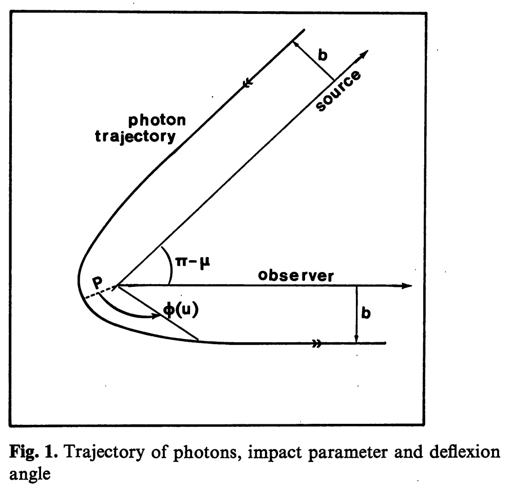
Equation (3) must be integrated over the range of values where \(u\) and \(G(u)\) are positive; i. e. between \(u_2\) and \(0\). Figure 1 shows the corresponding trajectory of the ray. We assume that \(r_0>> M\) is really at infinity (i. e. that the impact parameter on the plate is really \(b\), which is a good assumption), so that the final value, \(\varphi_\infty\), of \(\varphi\) is given by:

\[\varphi_\infty = \frac{1}{\sqrt{2M}}\int^{u_2}_0\frac{dx}{\sqrt{G(x)}}\quad(5a)\]

This integral can be transformed into a classical Jacobian elliptic integral (See derivation of equations 4,5 and 6)

\[\begin{aligned} \varphi_\infty &= 2\left(\frac{P}{Q}\right)^{1/2}\int^{\pi/2}_{\zeta\infty}(1-\kappa^2\sin^2x)^{-1/2}dx = 2\left(\frac{P}{Q}\right)^{1/2} \left(K(\kappa)-F(\zeta\infty,\kappa)\right)\quad(6). \end{aligned}\]

Here, \(K(\kappa)\) is the complete elliptic integral of modulus

\[\kappa \equiv \left(Q-P\frac{6M}{2Q}\right)^{1/2}\]

and \(F(\zeta\infty.\kappa)\) is the elliptic integral of modulus \(\kappa\) and argument \(\zeta_\infty\) such that

\[\sin^2\zeta_\infty = \frac{Q-P+2M}{Q-P+6M}.\]

The total deviation of the light ray, \(\mu\), is given by \(\varphi_\infty=\frac{\pi}{2}+\frac{\mu}{2}\). It is interesting to give the formulas at the limit \(P>>M\) and \(P\rightarrow 3M\). For very large \(P\) (weak field approximation) we verify immediately that \(\mu\sim 4M/P\), \(P\rightarrow b\) (See the derivation here). This famous formula for the deflection of light ray in the gravitational field of a spherical star leads to the Rutherford limit for the differential cross-section \(\frac{d\sigma}{d\Omega}=\frac{b}{\sin{\mu}}\lvert\frac{db}{d\mu}\rvert\) (which is precisely the number of particles per unit solid angle \(d\Omega=2\pi\sin\mu d\mu\) collected by the observer); which is independent of the energy of the incident photons.

For \(P\) near the critical value \(3M\), i.e. for \(b\) near \(b_c\), the asymptotic expansion of the elliptic funtions for modulus \(\kappa\sim 1\) (Gradshteyn and Ryzhik, 1965) leads to the important relation:

\[b = 5.19695M+3.4823M e^{-\mu} \quad(7)\]

In fact, the particles that come off at a given angle \(\mu\) in clude not only those that have really been deflected by \(\mu\), also those that have been deflected by \(\mu+2\pi\), \(\mu+4\pi\), …, \(\mu+2n\pi\), etc. (an infinite series of contributions), and which correspond to the following impact parameters (See the derivation here):

\[\begin{aligned} b_0&=b_c+3.4823M e^{-\mu} & \text{(zero circuit)}\\ b_1&=b_c+3.4823M e^{-(\mu+2\pi)} & \text{(one circuit)}\\ ...&...\\ b_n&=b_c+3.4823M e^{-(\mu+2n\pi)} &\text{(two circuit)}\\\\ ...&...\\ b_\infty&=b_c & \text{(infinity circuits)}\\ \end{aligned}\]

We see that the nth order contribution to the differential cross section is proprotional to

\[\frac{db_n}{d\mu} = - 3.4823 M e^{-(\mu+2n\pi)}\quad(8)\]

Thus the total contribution of successive numbers of circuits is proportional to \(\sum^{\infty}_0e^{-2n\pi}=\frac{1}{1-e^{-2\pi}}\). Thus in practice the contribution for \(n\geq 2\) is really negligeble. We shall see bellow the observational consequences of this fact.

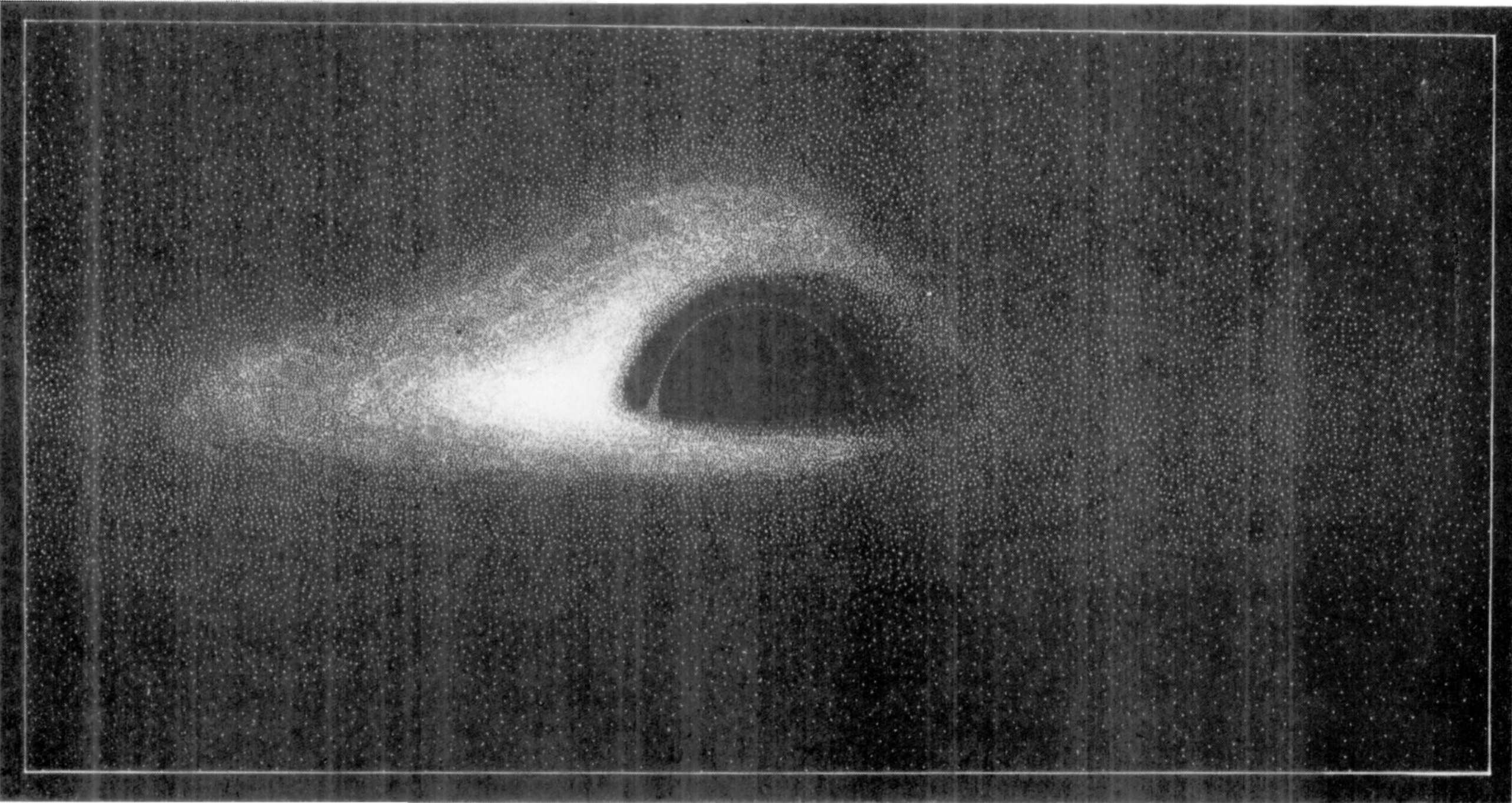
Once the properties of the deflectionangle \(\mu(b)\) are known, one is ready to work out what is the image of the black hole illuminatted by a parallel bean light, as seen by an observer placed on \(\Theta-\)direction. It follows from the above discussion that rays that reach the observer will give a picture consisting of a black disk of radius \(b_c= 5.19695M\) surrounded by ‘ghost’ rings of different radius and brightness. The exterior ring corresponds to the rays that have not described any circuit; as \(b\) approaches its critical value \(b_c\), the rays described more and more circuits, until in the limit \(b_\infty = b_c\) (infinite circuits) the rays are captured.

To conclue this section, the only ring practically distinguishable would be the external one. This is not a matter of brightness, but also a matter of resolution.

import warnings
warnings.filterwarnings('ignore')
'''
We began by defining the black hole mass M, the Schwarzschild radius r_s (horizon), 
the photon radius r_c (critical radius), the critical impact parameter b_c, and the function effective potential. 
We use geometrized units and create an arrange of values for r.
'''

def intensity_integrand(u):
    #Integral terms
    t1 = (1-2*M*u)**2
    t2 = 1/(1-b**2*u**2+2*M*b**2*u**3)
    return np.sqrt(t1*t2)

Denominator_intensity = lambda x: 1-b**2*x**2+2*M*b**2*x**3
Denominator = lambda x: (1/b**2)-x**2+2*M*x**3
b_intensity = np.arange(1e-3,20,1e-3)

I_o=np.zeros_like(b_intensity)

for i, b in enumerate(b_intensity):
    if b<b_c:
        specific_intensity = quad(intensity_integrand,0,1/2*M)[0]
        I_o[i]=specific_intensity
    else:
        uroot = float(optimize.fsolve(Denominator,0.15,xtol=1e-5))
        specific_intensity = quad(intensity_integrand,0, uroot)[0]
        I_o[i]=specific_intensity        

'''
Specific intensity function of b
'''
Io_interpol= make_interp_spline(b_intensity,I_o,k=3, t=None, bc_type=None, axis=0, check_finite=True)

plt.figure(figsize=(10, 10))
plt.plot(b_intensity,I_o,color= 'black')
plt.plot(-b_intensity,I_o,color='black')
plt.axvline(x=  b_c, color='black', linestyle=':', label='r = 10')
plt.axvline(x= -b_c, color='black', linestyle=':', label='r = 10')
#plt.plot(b_intensity,Io_interpol(b_intensity),'--',color='Red')
#plt.plot(-b_intensity,Io_interpol(b_intensity),'--',color='Red')
plt.title('Specific intensity')
plt.xlabel('b/M',fontsize=14)
plt.ylabel('$I_{obs}$',fontsize=14)
plt.xlim(-10,10)
plt.ylim(0.0,1)
plt.grid(True)

N = 1000
edge = 10
X = np.linspace(-edge,edge,N)
Y = np.linspace(-edge,edge,N)
b = np.zeros([N,N])
shadow_ring = np.zeros([N,N])

for j in range(len(X)):
    for i in range(len(Y)):
        b[i,j] = np.sqrt(X[i]**2 + Y[j]**2)
        shadow_ring[i,j] = Io_interpol(b[i,j])
maxv = shadow_ring.max()
minv = shadow_ring.min()

cmap = 'bone'#'gist_gray'
imgedge= edge
extent =[-imgedge, imgedge, -imgedge, imgedge]

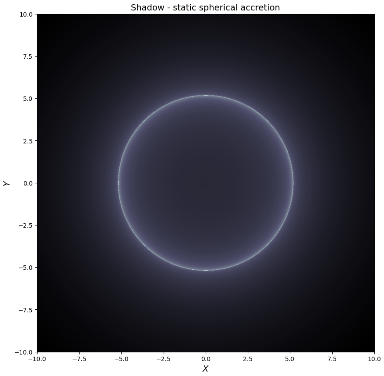
plt.figure(figsize=(10, 10))
plt.title('Shadow - static spherical accretion',fontsize=14)
plt.imshow(shadow_ring,cmap=cmap, origin='lower',vmax=maxv, vmin=minv, extent=extent)
plt.xlabel(r'$X$',fontsize=14)
plt.ylabel(r'$Y$',fontsize=14)

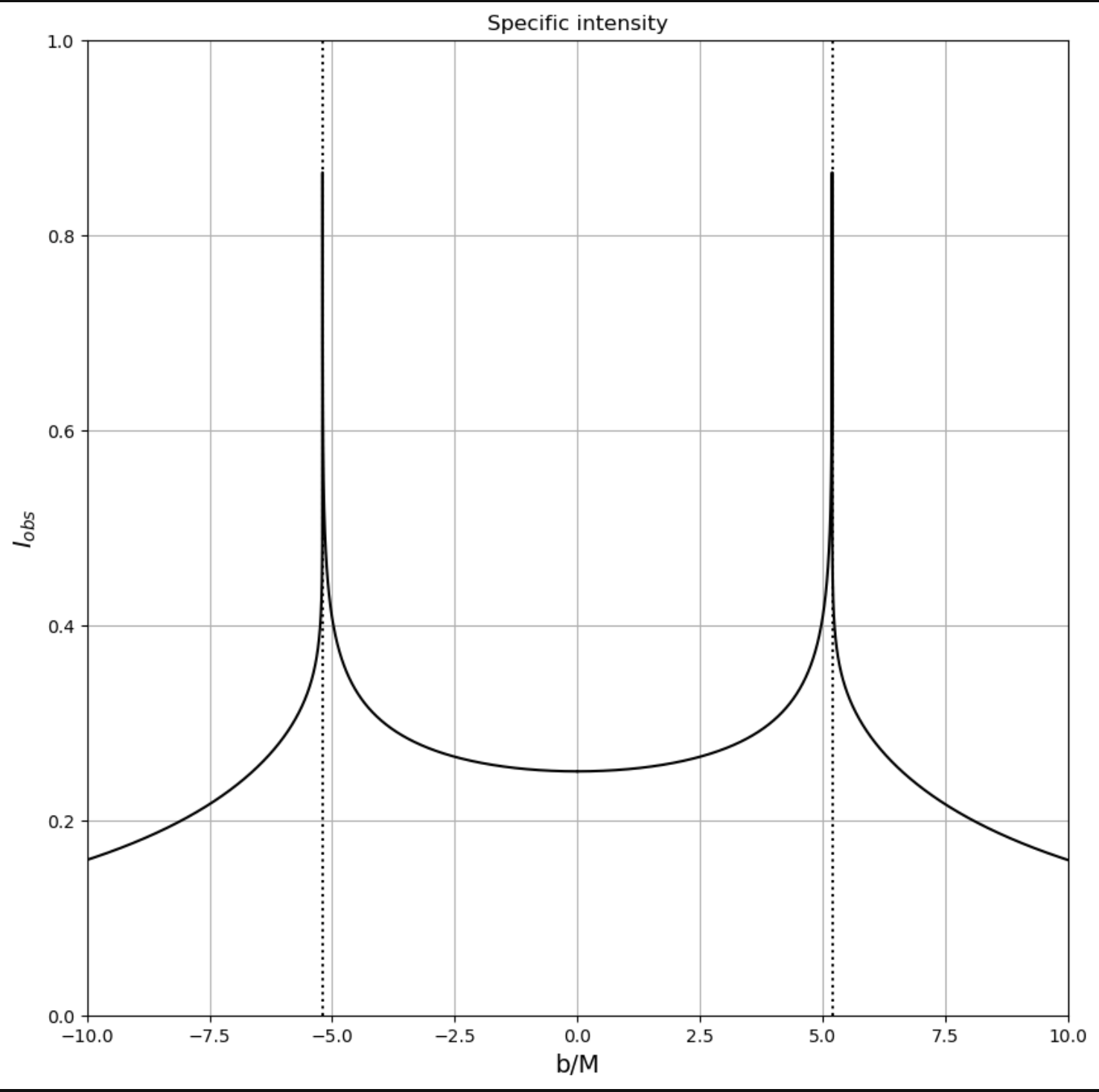
Especific intensity (static spherical accretion)	Shadow (static spherical accretion)

Images of Clothed Black holes

Let us now assume that the source of radiation is an emitting accretion disk orbiting arround the black hole; the astrophisical properties of such an object will be briefly discussed in the next section. Let the thickness of the disk be negligible with respect to M, so that it is considered as lying in the equatorial plane of the the Schwarzschild black hole. The coordinates system is chosen as in Figure. 3. The observver lies in the fixed direcion \(\theta_0\), \(\varphi_0=0\) (plane YOZ) at a distance \(r_0>>M\). We consider the disk as an assembly of idealized particles emitiing isotropically. Starting from an emitting partivle with Schwarzschild coordinates \((r,\varphi)\), a typical trajectory whose asymptotic direction is the observer’s direction OO’ lies in the plane OX’‘Y’’ and reaches the observer’s direction OO’ lies in the plane O’X’‘Y’ and reaches the photographic plate (which is the plane O’X’‘Y’’) at a point $m$, determined by its polar coordinates \((b,\alpha)\).

Assuming tha the observer is practically at infinity and at rest in the gravitational field of the black hole, then the polar distance from m to O’ is precisely the impact parameter of the trajectory, and the polar angle \(\alpha\), with the ‘‘vertical’’ direction O’Y’’ is the complement of the dihedral angle between planes OXY’ and OX’Y’. For a given coordinate \(r\), varying \(\varphi\) from 0 to \(\pi\) (the figure being symmetric with respect to O’Y’‘-axis), we get the apperent shape \(b(r)=b(r,\alpha)\) on the photographic plate of the circular ring orbiting the black hole at distance $r$.

As seen in the previous secton, rays emitted fro a given point M can circle around the black hole before escaping o infintiy, given an infinite series of images on the photographic plate; the same arguments indicate that only the secundary image (which corresponds to raus that have circuited once) has to be taken into account, images of higher order being emitter M, the observer will detect generally two images, a direct (or primary) image at polar coordinates \((b^{(d)},\alpha)\) and a gosh (or secundary) image at (\(b^{(g)},\alpha+\pi\)).

Relationships between the different angles involved by the problem follow directly from the resolution of spherical triangles $XMY’$ and $XMX’’$ (Fig 3). We get (See Derivation equations 9 and 10):

\[\cos \alpha = \frac{\cot \varphi \cos \theta_0}{\sin \gamma} = \frac{\cos \varphi \cos\theta_0}{\sqrt{1-\sin^2\theta_0\cos^2\varphi}}\quad(9).\]

So that \(\alpha\) is a monotonic function of \(\varphi\).

We need also the relation (See Derivation equations 9 and 10):

\[\cos\gamma=\cos\alpha\left(cos^2\alpha + \cot^2\theta_0\right)\quad(10).\]

Calculation of curves \(b^{(d)}(\alpha)\), \(b^{(g)}(\alpha)\) at fixed $r$ is performed with a computer. Nevertheless, prior to any precise drawing, we can foresee some characteristic features of the shape of our object by simply considering particular orbits in the plane \(\varphi=0\) for strong inclination (\(\theta_0=80^o\); Fig. 4). Already we can point out that one of the the main differences from the problem of the previous section is that not all orbits have necessarily a periastron, or equivalently an impact parameter greater than the critical value \(b_c\). For example, the trajectory 2 is emitted outside the horizon, at a distance \(2.60M\), and reaches the observer with an impact parameter \(b^{(d)}=4.75M\), lesser than \(b_c=5.20M\) (in fact, this trajectoy is only theoretically possible, but physically no photon will be emitted so near the horizon, see next section). More significant is the trajectory 3, which is emitted at \(r=9.80M\) from the the center of the hole but gives a direct image at only \(b^{(d)}=1.70M\). Clearly this is a pure projection effect, already encountered in a newtonian context when one observers Sturn’s rings near the equatorial plane. Furthermore, the very small values of \(b^{(d)}\) for trajectories emitted at relatively large $r$ but small \(\varphi\) imply that the orbits are almost purely radial (indeed trajectory 3 is very close to a straight line); thus, we expect the part of accretion disk between the hole and the observer to give direct images with the aspect of newtonian ellipses which project onto the lowe pat of the black spot. Figure 4 shows another characteristic feature of the shape: the secundary image is not everywhere in direct juxtaposition to the black hole spot of radius \(b_c\). In fact, trajectory 4 illustrates how, in order to reach the obsever at strong inclination, a photon emitted behind the hole necessarily suffers a weak deviation, and hence has an orbit with large periastron and impact parameter; so, we can presume that the secundary image is really dropped forward the observer’s direction (i. e. at relatively small values of \(\varphi\)), while on the opposite side it remains crushed around the black spot (at values of \(\varphi\) near \(\pi\)).

Enjoy reading this post while listen the Interstellar music!